2-2,三种计算图#
有三种计算图的构建方式:静态计算图,动态计算图,以及Autograph.
在TensorFlow1.0时代,采用的是静态计算图,需要先使用TensorFlow的各种算子创建计算图,然后再开启一个会话Session,显式执行计算图。
而在TensorFlow2.0时代,采用的是动态计算图,即每使用一个算子后,该算子会被动态加入到隐含的默认计算图中立即执行得到结果,而无需开启Session。
使用动态计算图即Eager Excution的好处是方便调试程序,它会让TensorFlow代码的表现和Python原生代码的表现一样,写起来就像写numpy一样,各种日志打印,控制流全部都是可以使用的。
使用动态计算图的缺点是运行效率相对会低一些。因为使用动态图会有许多次Python进程和TensorFlow的C++进程之间的通信。而静态计算图构建完成之后几乎全部在TensorFlow内核上使用C++代码执行,效率更高。此外静态图会对计算步骤进行一定的优化,剪去和结果无关的计算步骤。
如果需要在TensorFlow2.0中使用静态图,可以使用@tf.function装饰器将普通Python函数转换成对应的TensorFlow计算图构建代码。运行该函数就相当于在TensorFlow1.0中用Session执行代码。使用tf.function构建静态图的方式叫做 Autograph.
一,计算图简介#
计算图由节点(nodes)和线(edges)组成。
节点表示操作符Operator,或者称之为算子,线表示计算间的依赖。
实线表示有数据传递依赖,传递的数据即张量。
虚线通常可以表示控制依赖,即执行先后顺序。
二,静态计算图#
在TensorFlow1.0中,使用静态计算图分两步,第一步定义计算图,第二步在会话中执行计算图。
TensorFlow 1.0静态计算图范例
import tensorflow as tf

#定义计算图
g = tf.Graph()
with g.as_default():
    #placeholder为占位符,执行会话时候指定填充对象
    x = tf.placeholder(name='x', shape=[], dtype=tf.string)
    y = tf.placeholder(name='y', shape=[], dtype=tf.string)
    z = tf.string_join([x,y],name = 'join',separator=' ')

#执行计算图
with tf.Session(graph = g) as sess:
    print(sess.run(fetches = z,feed_dict = {x:"hello",y:"world"}))
TensorFlow2.0 怀旧版静态计算图
TensorFlow2.0为了确保对老版本tensorflow项目的兼容性,在tf.compat.v1子模块中保留了对TensorFlow1.0那种静态计算图构建风格的支持。
可称之为怀旧版静态计算图,已经不推荐使用了。
import tensorflow as tf

g = tf.compat.v1.Graph()
with g.as_default():
    x = tf.compat.v1.placeholder(name='x', shape=[], dtype=tf.string)
    y = tf.compat.v1.placeholder(name='y', shape=[], dtype=tf.string)
    z = tf.strings.join([x,y],name = "join",separator = " ")

with tf.compat.v1.Session(graph = g) as sess:
    # fetches的结果非常像一个函数的返回值,而feed_dict中的占位符相当于函数的参数序列。
    result = sess.run(fetches = z,feed_dict = {x:"hello",y:"world"})
    print(result)
b'hello world'
三,动态计算图#
在TensorFlow2.0中,使用的是动态计算图和Autograph.
在TensorFlow1.0中,使用静态计算图分两步,第一步定义计算图,第二步在会话中执行计算图。
动态计算图已经不区分计算图的定义和执行了,而是定义后立即执行。因此称之为 Eager Excution.
Eager这个英文单词的原意是"迫不及待的",也就是立即执行的意思。
# 动态计算图在每个算子处都进行构建,构建后立即执行

x = tf.constant("hello")
y = tf.constant("world")
z = tf.strings.join([x,y],separator=" ")

tf.print(z)
hello world
# 可以将动态计算图代码的输入和输出关系封装成函数

def strjoin(x,y):
    z =  tf.strings.join([x,y],separator = " ")
    tf.print(z)
    return z

result = strjoin(tf.constant("hello"),tf.constant("world"))
print(result)
hello world
tf.Tensor(b'hello world', shape=(), dtype=string)
四,TensorFlow2.0的Autograph#
动态计算图运行效率相对较低。
可以用@tf.function装饰器将普通Python函数转换成和TensorFlow1.0对应的静态计算图构建代码。
在TensorFlow1.0中,使用计算图分两步,第一步定义计算图,第二步在会话中执行计算图。
在TensorFlow2.0中,如果采用Autograph的方式使用计算图,第一步定义计算图变成了定义函数,第二步执行计算图变成了调用函数。
不需要使用会话了,一些都像原始的Python语法一样自然。
实践中,我们一般会先用动态计算图调试代码,然后在需要提高性能的的地方利用@tf.function切换成Autograph获得更高的效率。
当然,@tf.function的使用需要遵循一定的规范,我们后面章节将重点介绍。
import tensorflow as tf

# 使用autograph构建静态图

@tf.function
def strjoin(x,y):
    z =  tf.strings.join([x,y],separator = " ")
    tf.print(z)
    return z

result = strjoin(tf.constant("hello"),tf.constant("world"))

print(result)
hello world
tf.Tensor(b'hello world', shape=(), dtype=string)
import datetime

# 创建日志
import os
stamp = datetime.datetime.now().strftime("%Y%m%d-%H%M%S")
logdir = os.path.join('data', 'autograph', stamp)

## 在 Python3 下建议使用 pathlib 修正各操作系统的路径
# from pathlib import Path
# stamp = datetime.datetime.now().strftime("%Y%m%d-%H%M%S")
# logdir = str(Path('../../data/autograph/' + stamp))

writer = tf.summary.create_file_writer(logdir)

#开启autograph跟踪
tf.summary.trace_on(graph=True, profiler=True)

#执行autograph
result = strjoin("hello","world")

#将计算图信息写入日志
with writer.as_default():
    tf.summary.trace_export(
        name="autograph",
        step=0,
        profiler_outdir=logdir)
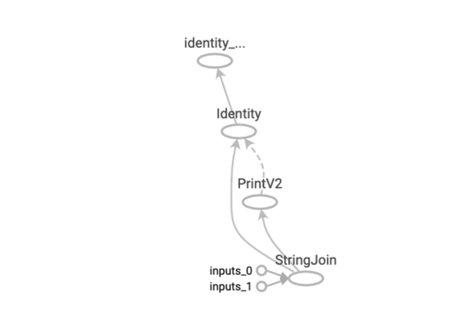
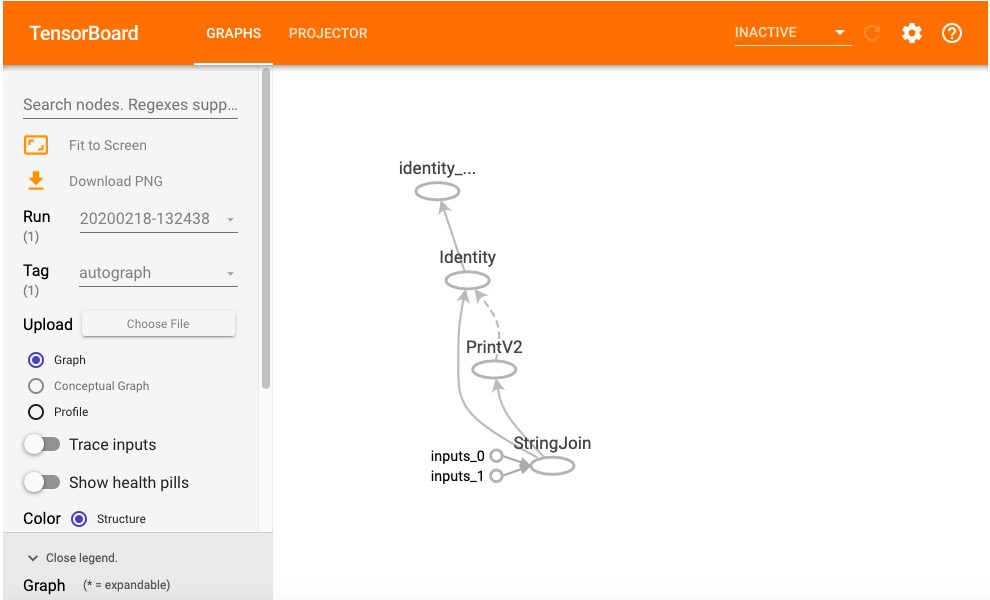
#启动 tensorboard在jupyter中的魔法命令
%load_ext tensorboard
#启动tensorboard
%tensorboard --logdir ../../data/autograph/
如果对本书内容理解上有需要进一步和作者交流的地方,欢迎在公众号"Python与算法之美"下留言。作者时间和精力有限,会酌情予以回复。
也可以在公众号后台回复关键字:加群,加入读者交流群和大家讨论。