3-2,中阶API示范#
下面的范例使用TensorFlow的中阶API实现线性回归模型和和DNN二分类模型。
TensorFlow的中阶API主要包括各种模型层,损失函数,优化器,数据管道,特征列等等。
import tensorflow as tf

#打印时间分割线
@tf.function
def printbar():
    today_ts = tf.timestamp()%(24*60*60)

    hour = tf.cast(today_ts//3600+8,tf.int32)%tf.constant(24)
    minite = tf.cast((today_ts%3600)//60,tf.int32)
    second = tf.cast(tf.floor(today_ts%60),tf.int32)

    def timeformat(m):
        if tf.strings.length(tf.strings.format("{}",m))==1:
            return(tf.strings.format("0{}",m))
        else:
            return(tf.strings.format("{}",m))

    timestring = tf.strings.join([timeformat(hour),timeformat(minite),
                timeformat(second)],separator = ":")
    tf.print("=========="*8+timestring)
一,线性回归模型#
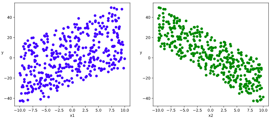
1,准备数据
import numpy as np
import pandas as pd
from matplotlib import pyplot as plt
import tensorflow as tf
from tensorflow.keras import layers,losses,metrics,optimizers

#样本数量
n = 400

# 生成测试用数据集
X = tf.random.uniform([n,2],minval=-10,maxval=10)
w0 = tf.constant([[2.0],[-3.0]])
b0 = tf.constant([[3.0]])
Y = X@w0 + b0 + tf.random.normal([n,1],mean = 0.0,stddev= 2.0)  # @表示矩阵乘法,增加正态扰动
# 数据可视化
%matplotlib inline
%config InlineBackend.figure_format = 'svg'
plt.figure(figsize = (12,5))
ax1 = plt.subplot(121)
ax1.scatter(X[:,0],Y[:,0], c = "b")
plt.xlabel("x1")
plt.ylabel("y",rotation = 0)

ax2 = plt.subplot(122)
ax2.scatter(X[:,1],Y[:,0], c = "g")
plt.xlabel("x2")
plt.ylabel("y",rotation = 0)
plt.show()
#构建输入数据管道
ds = tf.data.Dataset.from_tensor_slices((X,Y)) \
     .shuffle(buffer_size = 100).batch(10) \
     .prefetch(tf.data.experimental.AUTOTUNE)
2,定义模型
model = layers.Dense(units = 1)
model.build(input_shape = (2,)) #用build方法创建variables
model.loss_func = losses.mean_squared_error
model.optimizer = optimizers.SGD(learning_rate=0.001)
3,训练模型
#使用autograph机制转换成静态图加速

@tf.function
def train_step(model, features, labels):
    with tf.GradientTape() as tape:
        predictions = model(features)
        loss = model.loss_func(tf.reshape(labels,[-1]), tf.reshape(predictions,[-1]))
    grads = tape.gradient(loss,model.variables)
    model.optimizer.apply_gradients(zip(grads,model.variables))
    return loss

# 测试train_step效果
features,labels = next(ds.as_numpy_iterator())
train_step(model,features,labels)
def train_model(model,epochs):
    for epoch in tf.range(1,epochs+1):
        loss = tf.constant(0.0)
        for features, labels in ds:
            loss = train_step(model,features,labels)
        if epoch%50==0:
            printbar()
            tf.print("epoch =",epoch,"loss = ",loss)
            tf.print("w =",model.variables[0])
            tf.print("b =",model.variables[1])
train_model(model,epochs = 200)
================================================================================17:01:48
epoch = 50 loss =  2.56481647
w = [[1.99355531]
 [-2.99061537]]
b = [3.09484935]
================================================================================17:01:51
epoch = 100 loss =  5.96198225
w = [[1.98028314]
 [-2.96975136]]
b = [3.09501529]
================================================================================17:01:54
epoch = 150 loss =  4.79625702
w = [[2.00056171]
 [-2.98774862]]
b = [3.09567738]
================================================================================17:01:58
epoch = 200 loss =  8.26704407
w = [[2.00282311]
 [-2.99300027]]
b = [3.09406662]
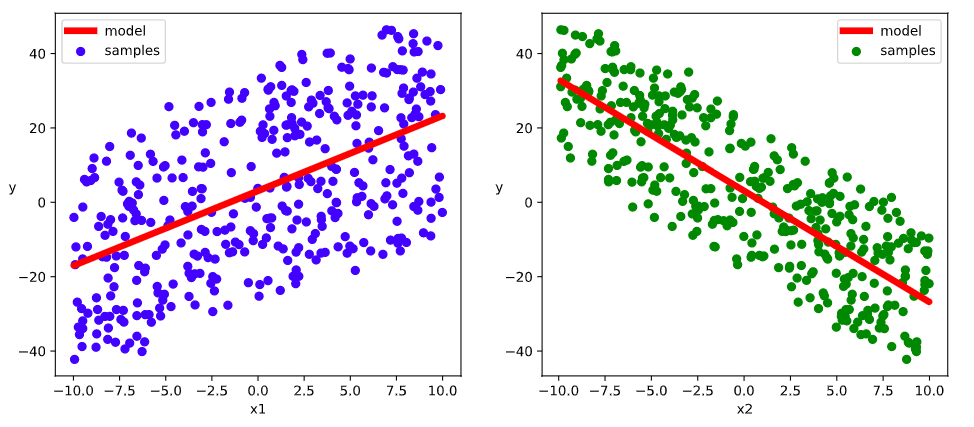
# 结果可视化

%matplotlib inline
%config InlineBackend.figure_format = 'svg'

w,b = model.variables

plt.figure(figsize = (12,5))
ax1 = plt.subplot(121)
ax1.scatter(X[:,0],Y[:,0], c = "b",label = "samples")
ax1.plot(X[:,0],w[0]*X[:,0]+b[0],"-r",linewidth = 5.0,label = "model")
ax1.legend()
plt.xlabel("x1")
plt.ylabel("y",rotation = 0)


ax2 = plt.subplot(122)
ax2.scatter(X[:,1],Y[:,0], c = "g",label = "samples")
ax2.plot(X[:,1],w[1]*X[:,1]+b[0],"-r",linewidth = 5.0,label = "model")
ax2.legend()
plt.xlabel("x2")
plt.ylabel("y",rotation = 0)

plt.show()
二, DNN二分类模型#
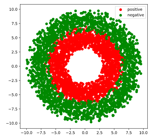
1,准备数据
import numpy as np
import pandas as pd
from matplotlib import pyplot as plt
import tensorflow as tf
from tensorflow.keras import layers,losses,metrics,optimizers
%matplotlib inline
%config InlineBackend.figure_format = 'svg'

#正负样本数量
n_positive,n_negative = 2000,2000

#生成正样本, 小圆环分布
r_p = 5.0 + tf.random.truncated_normal([n_positive,1],0.0,1.0)
theta_p = tf.random.uniform([n_positive,1],0.0,2*np.pi)
Xp = tf.concat([r_p*tf.cos(theta_p),r_p*tf.sin(theta_p)],axis = 1)
Yp = tf.ones_like(r_p)

#生成负样本, 大圆环分布
r_n = 8.0 + tf.random.truncated_normal([n_negative,1],0.0,1.0)
theta_n = tf.random.uniform([n_negative,1],0.0,2*np.pi)
Xn = tf.concat([r_n*tf.cos(theta_n),r_n*tf.sin(theta_n)],axis = 1)
Yn = tf.zeros_like(r_n)

#汇总样本
X = tf.concat([Xp,Xn],axis = 0)
Y = tf.concat([Yp,Yn],axis = 0)


#可视化
plt.figure(figsize = (6,6))
plt.scatter(Xp[:,0].numpy(),Xp[:,1].numpy(),c = "r")
plt.scatter(Xn[:,0].numpy(),Xn[:,1].numpy(),c = "g")
plt.legend(["positive","negative"]);
#构建输入数据管道
ds = tf.data.Dataset.from_tensor_slices((X,Y)) \
     .shuffle(buffer_size = 4000).batch(100) \
     .prefetch(tf.data.experimental.AUTOTUNE)
2, 定义模型
class DNNModel(tf.Module):
    def __init__(self,name = None):
        super(DNNModel, self).__init__(name=name)
        self.dense1 = layers.Dense(4,activation = "relu")
        self.dense2 = layers.Dense(8,activation = "relu")
        self.dense3 = layers.Dense(1,activation = "sigmoid")


    # 正向传播
    @tf.function(input_signature=[tf.TensorSpec(shape = [None,2], dtype = tf.float32)])
    def __call__(self,x):
        x = self.dense1(x)
        x = self.dense2(x)
        y = self.dense3(x)
        return y

model = DNNModel()
model.loss_func = losses.binary_crossentropy
model.metric_func = metrics.binary_accuracy
model.optimizer = optimizers.Adam(learning_rate=0.001)
# 测试模型结构
(features,labels) = next(ds.as_numpy_iterator())

predictions = model(features)

loss = model.loss_func(tf.reshape(labels,[-1]),tf.reshape(predictions,[-1]))
metric = model.metric_func(tf.reshape(labels,[-1]),tf.reshape(predictions,[-1]))

tf.print("init loss:",loss)
tf.print("init metric",metric)
init loss: 1.13653195
init metric 0.5
3,训练模型
#使用autograph机制转换成静态图加速

@tf.function
def train_step(model, features, labels):
    with tf.GradientTape() as tape:
        predictions = model(features)
        loss = model.loss_func(tf.reshape(labels,[-1]), tf.reshape(predictions,[-1]))
    grads = tape.gradient(loss,model.trainable_variables)
    model.optimizer.apply_gradients(zip(grads,model.trainable_variables))

    metric = model.metric_func(tf.reshape(labels,[-1]), tf.reshape(predictions,[-1]))

    return loss,metric

# 测试train_step效果
features,labels = next(ds.as_numpy_iterator())
train_step(model,features,labels)
(<tf.Tensor: shape=(), dtype=float32, numpy=1.2033114>,
 <tf.Tensor: shape=(), dtype=float32, numpy=0.47>)
def train_model(model,epochs):
    for epoch in tf.range(1,epochs+1):
        loss, metric = tf.constant(0.0),tf.constant(0.0)
        for features, labels in ds:
            loss,metric = train_step(model,features,labels)
        if epoch%10==0:
            printbar()
            tf.print("epoch =",epoch,"loss = ",loss, "accuracy = ",metric)
train_model(model,epochs = 60)
================================================================================17:07:36
epoch = 10 loss =  0.556449413 accuracy =  0.79
================================================================================17:07:38
epoch = 20 loss =  0.439187407 accuracy =  0.86
================================================================================17:07:40
epoch = 30 loss =  0.259921253 accuracy =  0.95
================================================================================17:07:42
epoch = 40 loss =  0.244920313 accuracy =  0.9
================================================================================17:07:43
epoch = 50 loss =  0.19839409 accuracy =  0.92
================================================================================17:07:45
epoch = 60 loss =  0.126151696 accuracy =  0.95
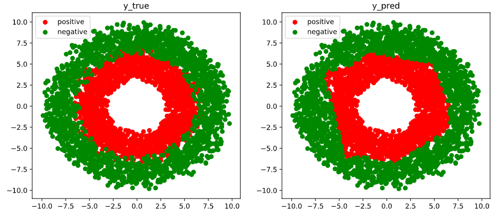
# 结果可视化
fig, (ax1,ax2) = plt.subplots(nrows=1,ncols=2,figsize = (12,5))
ax1.scatter(Xp[:,0].numpy(),Xp[:,1].numpy(),c = "r")
ax1.scatter(Xn[:,0].numpy(),Xn[:,1].numpy(),c = "g")
ax1.legend(["positive","negative"]);
ax1.set_title("y_true");

Xp_pred = tf.boolean_mask(X,tf.squeeze(model(X)>=0.5),axis = 0)
Xn_pred = tf.boolean_mask(X,tf.squeeze(model(X)<0.5),axis = 0)

ax2.scatter(Xp_pred[:,0].numpy(),Xp_pred[:,1].numpy(),c = "r")
ax2.scatter(Xn_pred[:,0].numpy(),Xn_pred[:,1].numpy(),c = "g")
ax2.legend(["positive","negative"]);
ax2.set_title("y_pred");
如果对本书内容理解上有需要进一步和作者交流的地方,欢迎在公众号"Python与算法之美"下留言。作者时间和精力有限,会酌情予以回复。
也可以在公众号后台回复关键字:加群,加入读者交流群和大家讨论。