3-3 High-level API: Demonstration#
The examples below use high-level APIs in TensorFlow to implement a linear regression model and a DNN binary classification model.
Typically, the high-level APIs are providing the class interfaces for tf.keras.models.
There are three ways of modeling using APIs of Keras: sequential modeling using Sequential function, arbitrary modeling using API functions, and customized modeling by inheriting base class Model.
Here we are demonstrating using Sequential function and customized modeling by inheriting base class Model, respectively.
import tensorflow as tf

# Time stamp
@tf.function
def printbar():
    today_ts = tf.timestamp()%(24*60*60)

    hour = tf.cast(today_ts//3600+8,tf.int32)%tf.constant(24)
    minite = tf.cast((today_ts%3600)//60,tf.int32)
    second = tf.cast(tf.floor(today_ts%60),tf.int32)

    def timeformat(m):
        if tf.strings.length(tf.strings.format("{}",m))==1:
            return(tf.strings.format("0{}",m))
        else:
            return(tf.strings.format("{}",m))

    timestring = tf.strings.join([timeformat(hour),timeformat(minite),
                timeformat(second)],separator = ":")
    tf.print("=========="*8+timestring)
1. Linear Regression Model#
In this example, we used Sequential function to construct the model sequentially and use the pre-defined method model.fit for training (for the beginners).
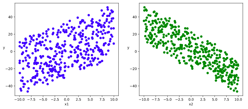
(a) Data Preparation
import numpy as np
import pandas as pd
from matplotlib import pyplot as plt
import tensorflow as tf
from tensorflow.keras import models,layers,losses,metrics,optimizers

# Number of sample
n = 400

# Generating the datasets
X = tf.random.uniform([n,2],minval=-10,maxval=10)
w0 = tf.constant([[2.0],[-3.0]])
b0 = tf.constant([[3.0]])
Y = X@w0 + b0 + tf.random.normal([n,1],mean = 0.0,stddev= 2.0)  # @ is matrix multiplication; adding Gaussian noise
# Data Visualization

%matplotlib inline
%config InlineBackend.figure_format = 'svg'
plt.figure(figsize = (12,5))
ax1 = plt.subplot(121)
ax1.scatter(X[:,0],Y[:,0], c = "b")
plt.xlabel("x1")
plt.ylabel("y",rotation = 0)

ax2 = plt.subplot(122)
ax2.scatter(X[:,1],Y[:,0], c = "g")
plt.xlabel("x2")
plt.ylabel("y",rotation = 0)
plt.show()
(b) Model Definition
tf.keras.backend.clear_session()

model = models.Sequential()
model.add(layers.Dense(1,input_shape =(2,)))
model.summary()
Model: "sequential"
_________________________________________________________________
Layer (type)                 Output Shape              Param #
=================================================================
dense (Dense)                (None, 1)                 3
=================================================================
Total params: 3
Trainable params: 3
Non-trainable params: 0
© Model Training
### Training using method fit

model.compile(optimizer="adam",loss="mse",metrics=["mae"])
model.fit(X,Y,batch_size = 10,epochs = 200)

tf.print("w = ",model.layers[0].kernel)
tf.print("b = ",model.layers[0].bias)
Epoch 197/200
400/400 [==============================] - 0s 190us/sample - loss: 4.3977 - mae: 1.7129
Epoch 198/200
400/400 [==============================] - 0s 172us/sample - loss: 4.3918 - mae: 1.7117
Epoch 199/200
400/400 [==============================] - 0s 134us/sample - loss: 4.3861 - mae: 1.7106
Epoch 200/200
400/400 [==============================] - 0s 166us/sample - loss: 4.3786 - mae: 1.7092
w =  [[1.99339032]
 [-3.00866461]]
b =  [2.67018795]
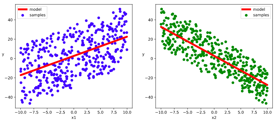
# Visualizing the results

%matplotlib inline
%config InlineBackend.figure_format = 'svg'

w,b = model.variables

plt.figure(figsize = (12,5))
ax1 = plt.subplot(121)
ax1.scatter(X[:,0],Y[:,0], c = "b",label = "samples")
ax1.plot(X[:,0],w[0]*X[:,0]+b[0],"-r",linewidth = 5.0,label = "model")
ax1.legend()
plt.xlabel("x1")
plt.ylabel("y",rotation = 0)

ax2 = plt.subplot(122)
ax2.scatter(X[:,1],Y[:,0], c = "g",label = "samples")
ax2.plot(X[:,1],w[1]*X[:,1]+b[0],"-r",linewidth = 5.0,label = "model")
ax2.legend()
plt.xlabel("x2")
plt.ylabel("y",rotation = 0)

plt.show()
2. DNN Binary Classification Model#
This example demonstrates the customized model using the child class inherited from the base class Model, and use a customized loop for training (for the experts).
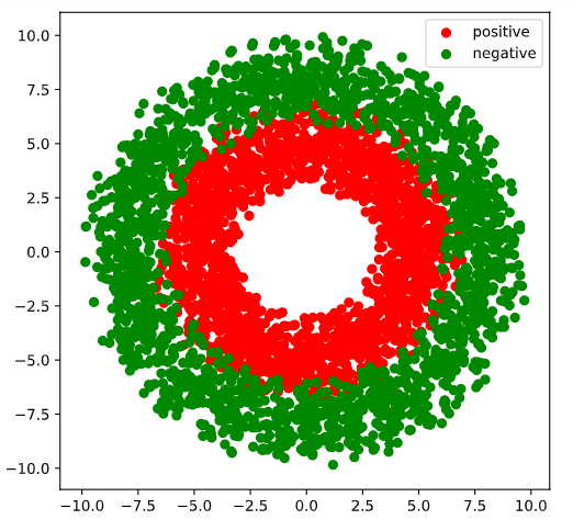
(a) Data Preparation
import numpy as np
import pandas as pd
from matplotlib import pyplot as plt
import tensorflow as tf
from tensorflow.keras import layers,losses,metrics,optimizers
%matplotlib inline
%config InlineBackend.figure_format = 'svg'

# Number of the positive/negative samples
n_positive,n_negative = 2000,2000

# Generating the positive samples with a distribution on a smaller ring
r_p = 5.0 + tf.random.truncated_normal([n_positive,1],0.0,1.0)
theta_p = tf.random.uniform([n_positive,1],0.0,2*np.pi)
Xp = tf.concat([r_p*tf.cos(theta_p),r_p*tf.sin(theta_p)],axis = 1)
Yp = tf.ones_like(r_p)

# Generating the negative samples with a distribution on a larger ring
r_n = 8.0 + tf.random.truncated_normal([n_negative,1],0.0,1.0)
theta_n = tf.random.uniform([n_negative,1],0.0,2*np.pi)
Xn = tf.concat([r_n*tf.cos(theta_n),r_n*tf.sin(theta_n)],axis = 1)
Yn = tf.zeros_like(r_n)

# Assembling all samples
X = tf.concat([Xp,Xn],axis = 0)
Y = tf.concat([Yp,Yn],axis = 0)

# Shuffling the samples
data = tf.concat([X,Y],axis = 1)
data = tf.random.shuffle(data)
X = data[:,:2]
Y = data[:,2:]


# Visualizing the data
plt.figure(figsize = (6,6))
plt.scatter(Xp[:,0].numpy(),Xp[:,1].numpy(),c = "r")
plt.scatter(Xn[:,0].numpy(),Xn[:,1].numpy(),c = "g")
plt.legend(["positive","negative"]);
ds_train = tf.data.Dataset.from_tensor_slices((X[0:n*3//4,:],Y[0:n*3//4,:])) \
     .shuffle(buffer_size = 1000).batch(20) \
     .prefetch(tf.data.experimental.AUTOTUNE) \
     .cache()

ds_valid = tf.data.Dataset.from_tensor_slices((X[n*3//4:,:],Y[n*3//4:,:])) \
     .batch(20) \
     .prefetch(tf.data.experimental.AUTOTUNE) \
     .cache()
(b) Model Definition
tf.keras.backend.clear_session()
class DNNModel(models.Model):
    def __init__(self):
        super(DNNModel, self).__init__()

    def build(self,input_shape):
        self.dense1 = layers.Dense(4,activation = "relu",name = "dense1")
        self.dense2 = layers.Dense(8,activation = "relu",name = "dense2")
        self.dense3 = layers.Dense(1,activation = "sigmoid",name = "dense3")
        super(DNNModel,self).build(input_shape)

    # Forward propagation
    @tf.function(input_signature=[tf.TensorSpec(shape = [None,2], dtype = tf.float32)])
    def call(self,x):
        x = self.dense1(x)
        x = self.dense2(x)
        y = self.dense3(x)
        return y

model = DNNModel()
model.build(input_shape =(None,2))

model.summary()
Model: "dnn_model"
_________________________________________________________________
Layer (type)                 Output Shape              Param #
=================================================================
dense1 (Dense)               multiple                  12
_________________________________________________________________
dense2 (Dense)               multiple                  40
_________________________________________________________________
dense3 (Dense)               multiple                  9
=================================================================
Total params: 61
Trainable params: 61
Non-trainable params: 0
_________________________________________________________________
© Model Training
### Customizing the training loop

optimizer = optimizers.Adam(learning_rate=0.01)
loss_func = tf.keras.losses.BinaryCrossentropy()

train_loss = tf.keras.metrics.Mean(name='train_loss')
train_metric = tf.keras.metrics.BinaryAccuracy(name='train_accuracy')

valid_loss = tf.keras.metrics.Mean(name='valid_loss')
valid_metric = tf.keras.metrics.BinaryAccuracy(name='valid_accuracy')


@tf.function
def train_step(model, features, labels):
    with tf.GradientTape() as tape:
        predictions = model(features)
        loss = loss_func(labels, predictions)
    grads = tape.gradient(loss, model.trainable_variables)
    optimizer.apply_gradients(zip(grads, model.trainable_variables))

    train_loss.update_state(loss)
    train_metric.update_state(labels, predictions)

@tf.function
def valid_step(model, features, labels):
    predictions = model(features)
    batch_loss = loss_func(labels, predictions)
    valid_loss.update_state(batch_loss)
    valid_metric.update_state(labels, predictions)


def train_model(model,ds_train,ds_valid,epochs):
    for epoch in tf.range(1,epochs+1):
        for features, labels in ds_train:
            train_step(model,features,labels)

        for features, labels in ds_valid:
            valid_step(model,features,labels)

        logs = 'Epoch={},Loss:{},Accuracy:{},Valid Loss:{},Valid Accuracy:{}'

        if  epoch%100 ==0:
            printbar()
            tf.print(tf.strings.format(logs,
            (epoch,train_loss.result(),train_metric.result(),valid_loss.result(),valid_metric.result())))

        train_loss.reset_states()
        valid_loss.reset_states()
        train_metric.reset_states()
        valid_metric.reset_states()

train_model(model,ds_train,ds_valid,1000)
================================================================================17:35:02
Epoch=100,Loss:0.194088802,Accuracy:0.923064,Valid Loss:0.215538561,Valid Accuracy:0.904368
================================================================================17:35:22
Epoch=200,Loss:0.151239693,Accuracy:0.93768847,Valid Loss:0.181166962,Valid Accuracy:0.920664132
================================================================================17:35:43
Epoch=300,Loss:0.134556711,Accuracy:0.944247484,Valid Loss:0.171530813,Valid Accuracy:0.926396072
================================================================================17:36:04
Epoch=400,Loss:0.125722557,Accuracy:0.949172914,Valid Loss:0.16731061,Valid Accuracy:0.929318547
================================================================================17:36:24
Epoch=500,Loss:0.120216407,Accuracy:0.952525079,Valid Loss:0.164817035,Valid Accuracy:0.931044817
================================================================================17:36:44
Epoch=600,Loss:0.116434008,Accuracy:0.954830289,Valid Loss:0.163089141,Valid Accuracy:0.932202339
================================================================================17:37:05
Epoch=700,Loss:0.113658346,Accuracy:0.956433,Valid Loss:0.161804497,Valid Accuracy:0.933092058
================================================================================17:37:25
Epoch=800,Loss:0.111522928,Accuracy:0.957467675,Valid Loss:0.160796657,Valid Accuracy:0.93379426
================================================================================17:37:46
Epoch=900,Loss:0.109816991,Accuracy:0.958205402,Valid Loss:0.159987748,Valid Accuracy:0.934343576
================================================================================17:38:06
Epoch=1000,Loss:0.10841465,Accuracy:0.958805501,Valid Loss:0.159325734,Valid Accuracy:0.934785843
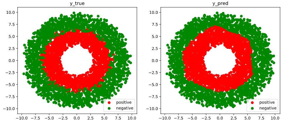
# Visualizing the results
fig, (ax1,ax2) = plt.subplots(nrows=1,ncols=2,figsize = (12,5))
ax1.scatter(Xp[:,0].numpy(),Xp[:,1].numpy(),c = "r")
ax1.scatter(Xn[:,0].numpy(),Xn[:,1].numpy(),c = "g")
ax1.legend(["positive","negative"]);
ax1.set_title("y_true");

Xp_pred = tf.boolean_mask(X,tf.squeeze(model(X)>=0.5),axis = 0)
Xn_pred = tf.boolean_mask(X,tf.squeeze(model(X)<0.5),axis = 0)

ax2.scatter(Xp_pred[:,0].numpy(),Xp_pred[:,1].numpy(),c = "r")
ax2.scatter(Xn_pred[:,0].numpy(),Xn_pred[:,1].numpy(),c = "g")
ax2.legend(["positive","negative"]);
ax2.set_title("y_pred");
Please leave comments in the WeChat official account "Python与算法之美" (Elegance of Python and Algorithms) if you want to communicate with the author about the content. The author will try best to reply given the limited time available.
You are also welcomed to join the group chat with the other readers through replying 加群 (join group) in the WeChat official account.