3-2 Mid-level API: Demonstration#
The examples below use mid-level APIs in TensorFlow to implement a linear regression model and a DNN binary classification model.
Mid-level API includes model layers, loss functions, optimizers, data pipelines, feature columns, etc.
import tensorflow as tf

# Time stamp
@tf.function
def printbar():
    today_ts = tf.timestamp()%(24*60*60)

    hour = tf.cast(today_ts//3600+8,tf.int32)%tf.constant(24)
    minite = tf.cast((today_ts%3600)//60,tf.int32)
    second = tf.cast(tf.floor(today_ts%60),tf.int32)

    def timeformat(m):
        if tf.strings.length(tf.strings.format("{}",m))==1:
            return(tf.strings.format("0{}",m))
        else:
            return(tf.strings.format("{}",m))

    timestring = tf.strings.join([timeformat(hour),timeformat(minite),
                timeformat(second)],separator = ":")
    tf.print("=========="*8+timestring)
1. Linear Regression Model#
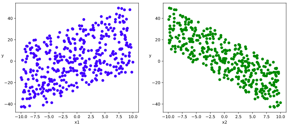
(a) Data Preparation
import numpy as np
import pandas as pd
from matplotlib import pyplot as plt
import tensorflow as tf
from tensorflow.keras import layers,losses,metrics,optimizers

# Number of sample
n = 400

# Generating the datasets
X = tf.random.uniform([n,2],minval=-10,maxval=10)
w0 = tf.constant([[2.0],[-3.0]])
b0 = tf.constant([[3.0]])
Y = X@w0 + b0 + tf.random.normal([n,1],mean = 0.0,stddev= 2.0)  # @ is matrix multiplication; adding Gaussian noise
# Data Visualization
%matplotlib inline
%config InlineBackend.figure_format = 'svg'
plt.figure(figsize = (12,5))
ax1 = plt.subplot(121)
ax1.scatter(X[:,0],Y[:,0], c = "b")
plt.xlabel("x1")
plt.ylabel("y",rotation = 0)

ax2 = plt.subplot(122)
ax2.scatter(X[:,1],Y[:,0], c = "g")
plt.xlabel("x2")
plt.ylabel("y",rotation = 0)
plt.show()
# Creating generator of data pipeline
ds = tf.data.Dataset.from_tensor_slices((X,Y)) \
     .shuffle(buffer_size = 100).batch(10) \
     .prefetch(tf.data.experimental.AUTOTUNE)
(b) Model Definition
model = layers.Dense(units = 1)
model.build(input_shape = (2,)) #Creating variables using the build method
model.loss_func = losses.mean_squared_error
model.optimizer = optimizers.SGD(learning_rate=0.001)
© Model Training
# Accelerate using Autograph to transform the dynamic graph into static

@tf.function
def train_step(model, features, labels):
    with tf.GradientTape() as tape:
        predictions = model(features)
        loss = model.loss_func(tf.reshape(labels,[-1]), tf.reshape(predictions,[-1]))
    grads = tape.gradient(loss,model.variables)
    model.optimizer.apply_gradients(zip(grads,model.variables))
    return loss

# Testing the results of train_step
features,labels = next(ds.as_numpy_iterator())
train_step(model,features,labels)
def train_model(model,epochs):
    for epoch in tf.range(1,epochs+1):
        loss = tf.constant(0.0)
        for features, labels in ds:
            loss = train_step(model,features,labels)
        if epoch%50==0:
            printbar()
            tf.print("epoch =",epoch,"loss = ",loss)
            tf.print("w =",model.variables[0])
            tf.print("b =",model.variables[1])
train_model(model,epochs = 200)
================================================================================17:01:48
epoch = 50 loss =  2.56481647
w = [[1.99355531]
 [-2.99061537]]
b = [3.09484935]
================================================================================17:01:51
epoch = 100 loss =  5.96198225
w = [[1.98028314]
 [-2.96975136]]
b = [3.09501529]
================================================================================17:01:54
epoch = 150 loss =  4.79625702
w = [[2.00056171]
 [-2.98774862]]
b = [3.09567738]
================================================================================17:01:58
epoch = 200 loss =  8.26704407
w = [[2.00282311]
 [-2.99300027]]
b = [3.09406662]
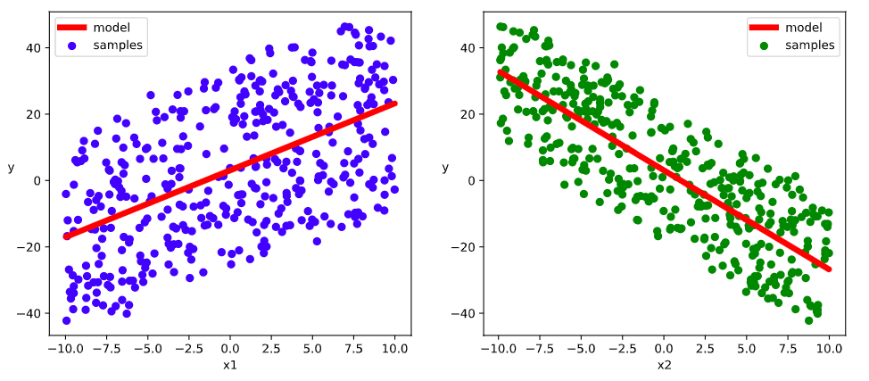
# Visualizing the results

%matplotlib inline
%config InlineBackend.figure_format = 'svg'

w,b = model.variables

plt.figure(figsize = (12,5))
ax1 = plt.subplot(121)
ax1.scatter(X[:,0],Y[:,0], c = "b",label = "samples")
ax1.plot(X[:,0],w[0]*X[:,0]+b[0],"-r",linewidth = 5.0,label = "model")
ax1.legend()
plt.xlabel("x1")
plt.ylabel("y",rotation = 0)


ax2 = plt.subplot(122)
ax2.scatter(X[:,1],Y[:,0], c = "g",label = "samples")
ax2.plot(X[:,1],w[1]*X[:,1]+b[0],"-r",linewidth = 5.0,label = "model")
ax2.legend()
plt.xlabel("x2")
plt.ylabel("y",rotation = 0)

plt.show()
2. DNN Binary Classification Model#
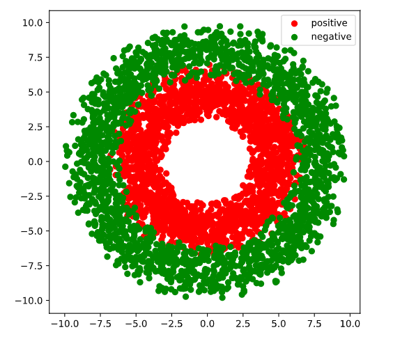
(a) Data Preparation
import numpy as np
import pandas as pd
from matplotlib import pyplot as plt
import tensorflow as tf
from tensorflow.keras import layers,losses,metrics,optimizers
%matplotlib inline
%config InlineBackend.figure_format = 'svg'

## Number of the positive/negative samples
n_positive,n_negative = 2000,2000

# Generating the positive samples with a distribution on a smaller ring
r_p = 5.0 + tf.random.truncated_normal([n_positive,1],0.0,1.0)
theta_p = tf.random.uniform([n_positive,1],0.0,2*np.pi)
Xp = tf.concat([r_p*tf.cos(theta_p),r_p*tf.sin(theta_p)],axis = 1)
Yp = tf.ones_like(r_p)

# Generating the negative samples with a distribution on a larger ring
r_n = 8.0 + tf.random.truncated_normal([n_negative,1],0.0,1.0)
theta_n = tf.random.uniform([n_negative,1],0.0,2*np.pi)
Xn = tf.concat([r_n*tf.cos(theta_n),r_n*tf.sin(theta_n)],axis = 1)
Yn = tf.zeros_like(r_n)

# Assembling all samples
X = tf.concat([Xp,Xn],axis = 0)
Y = tf.concat([Yp,Yn],axis = 0)


# Visualizing the data
plt.figure(figsize = (6,6))
plt.scatter(Xp[:,0].numpy(),Xp[:,1].numpy(),c = "r")
plt.scatter(Xn[:,0].numpy(),Xn[:,1].numpy(),c = "g")
plt.legend(["positive","negative"]);
# Create pipeline for the input data
ds = tf.data.Dataset.from_tensor_slices((X,Y)) \
     .shuffle(buffer_size = 4000).batch(100) \
     .prefetch(tf.data.experimental.AUTOTUNE)
(b) Model Definition
class DNNModel(tf.Module):
    def __init__(self,name = None):
        super(DNNModel, self).__init__(name=name)
        self.dense1 = layers.Dense(4,activation = "relu")
        self.dense2 = layers.Dense(8,activation = "relu")
        self.dense3 = layers.Dense(1,activation = "sigmoid")


    # Forward propagation
    @tf.function(input_signature=[tf.TensorSpec(shape = [None,2], dtype = tf.float32)])
    def __call__(self,x):
        x = self.dense1(x)
        x = self.dense2(x)
        y = self.dense3(x)
        return y

model = DNNModel()
model.loss_func = losses.binary_crossentropy
model.metric_func = metrics.binary_accuracy
model.optimizer = optimizers.Adam(learning_rate=0.001)
# Testing the structure of model
(features,labels) = next(ds.as_numpy_iterator())

predictions = model(features)

loss = model.loss_func(tf.reshape(labels,[-1]),tf.reshape(predictions,[-1]))
metric = model.metric_func(tf.reshape(labels,[-1]),tf.reshape(predictions,[-1]))

tf.print("init loss:",loss)
tf.print("init metric",metric)
init loss: 1.13653195
init metric 0.5
© Model Training
# Transform to static graph for acceleration using Autograph

@tf.function
def train_step(model, features, labels):
    with tf.GradientTape() as tape:
        predictions = model(features)
        loss = model.loss_func(tf.reshape(labels,[-1]), tf.reshape(predictions,[-1]))
    grads = tape.gradient(loss,model.trainable_variables)
    model.optimizer.apply_gradients(zip(grads,model.trainable_variables))

    metric = model.metric_func(tf.reshape(labels,[-1]), tf.reshape(predictions,[-1]))

    return loss,metric

# Testing the result of train_step
features,labels = next(ds.as_numpy_iterator())
train_step(model,features,labels)
(<tf.Tensor: shape=(), dtype=float32, numpy=1.2033114>,
 <tf.Tensor: shape=(), dtype=float32, numpy=0.47>)
@tf.function
def train_model(model,epochs):
    for epoch in tf.range(1,epochs+1):
        loss, metric = tf.constant(0.0),tf.constant(0.0)
        for features, labels in ds:
            loss,metric = train_step(model,features,labels)
        if epoch%10==0:
            printbar()
            tf.print("epoch =",epoch,"loss = ",loss, "accuracy = ",metric)
train_model(model,epochs = 60)
================================================================================17:07:36
epoch = 10 loss =  0.556449413 accuracy =  0.79
================================================================================17:07:38
epoch = 20 loss =  0.439187407 accuracy =  0.86
================================================================================17:07:40
epoch = 30 loss =  0.259921253 accuracy =  0.95
================================================================================17:07:42
epoch = 40 loss =  0.244920313 accuracy =  0.9
================================================================================17:07:43
epoch = 50 loss =  0.19839409 accuracy =  0.92
================================================================================17:07:45
epoch = 60 loss =  0.126151696 accuracy =  0.95
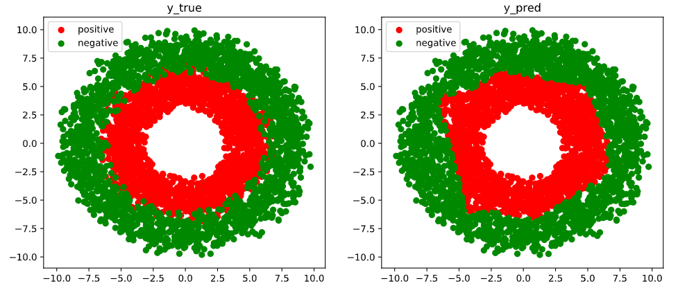
# Visualizing the results
fig, (ax1,ax2) = plt.subplots(nrows=1,ncols=2,figsize = (12,5))
ax1.scatter(Xp[:,0].numpy(),Xp[:,1].numpy(),c = "r")
ax1.scatter(Xn[:,0].numpy(),Xn[:,1].numpy(),c = "g")
ax1.legend(["positive","negative"]);
ax1.set_title("y_true");

Xp_pred = tf.boolean_mask(X,tf.squeeze(model(X)>=0.5),axis = 0)
Xn_pred = tf.boolean_mask(X,tf.squeeze(model(X)<0.5),axis = 0)

ax2.scatter(Xp_pred[:,0].numpy(),Xp_pred[:,1].numpy(),c = "r")
ax2.scatter(Xn_pred[:,0].numpy(),Xn_pred[:,1].numpy(),c = "g")
ax2.legend(["positive","negative"]);
ax2.set_title("y_pred");
Please leave comments in the WeChat official account "Python与算法之美" (Elegance of Python and Algorithms) if you want to communicate with the author about the content. The author will try best to reply given the limited time available.
You are also welcomed to join the group chat with the other readers through replying 加群 (join group) in the WeChat official account.